LOGISTIC REGRESSION (Titanic dataset)
Logistic regression is a techinque used for solving the classification problem and Classification is nothing but a problem of identifing to which of a set of categories a new observation belongs, on the basis of training dataset containing observations (or instances) whose categorical membership is known.
- 1. Problem Statement
- 2. Data Loading and Description
- 3. Preprocessing the data
- 4. Logistic Regression
- 4.2 Mathematics behind Logistic Regression
- 4.3 Applications of Logistic Regression
- 4.4 Preparing X and y using pandas
- 4.5 Splitting X and y into training and test datasets.
- 4.6 Logistic regression in scikit-learn
- 4.7 Using the Model for Prediction
- 5. Model evaluation
The goal is to predict survival of passengers travelling in RMS Titanic using Logistic regression.
- The dataset consists of the information about people boarding the famous RMS Titanic. Various variables present in the dataset includes data of age, sex, fare, ticket etc.
- The dataset comprises of 891 observations of 12 columns. Below is a table showing names of all the columns and their description.
| Column Name | Description |
|---|---|
| PassengerId | Passenger Identity |
| Survived | Whether passenger survived or not |
| Pclass | Class of ticket |
| Name | Name of passenger |
| Sex | Sex of passenger |
| Age | Age of passenger |
| SibSp | Number of sibling and/or spouse travelling with passenger |
| Parch | Number of parent and/or children travelling with passenger |
| Ticket | Ticket number |
| Fare | Price of ticket |
| Cabin | Cabin number |
import numpy as np                                                 # Implemennts milti-dimensional array and matrices
import pandas as pd                                                # For data manipulation and analysis
# import pandas_profiling
import matplotlib.pyplot as plt                                    # Plotting library for Python programming language and it's numerical mathematics extension NumPy
import seaborn as sns                                              # Provides a high level interface for drawing attractive and informative statistical graphics
%matplotlib inline
sns.set()

from subprocess import check_output
titanic_data = pd.read_csv("LogReg/titanic_train.csv") # Importing training dataset using pd.read_csv
- Dealing with missing values
- Dropping/Replacing missing entries of Embarked.
- Replacing missing values of Age and Fare with median values.
- Dropping the column 'Cabin' as it has too many null values.
titanic_data.Embarked = titanic_data.Embarked.fillna(titanic_data['Embarked'].mode()[0])
median_age = titanic_data.Age.median()
median_fare = titanic_data.Fare.median()
titanic_data.Age.fillna(median_age, inplace = True)
titanic_data.Fare.fillna(median_fare, inplace = True)
titanic_data.drop('Cabin', axis = 1,inplace = True)
- Creating a new feature named FamilySize.
titanic_data['FamilySize'] = titanic_data['SibSp'] + titanic_data['Parch']+1
- Segmenting Sex column as per Age, Age less than 15 as Child, Age greater than 15 as Males and Females as per their gender.
titanic_data['GenderClass'] = titanic_data.apply(lambda x: 'child' if x['Age'] < 15 else x['Sex'],axis=1)
titanic_data[titanic_data.Age<15].head(2)
titanic_data[titanic_data.Age>15].head(2)
- Dummification of GenderClass & Embarked.
titanic_data = pd.get_dummies(titanic_data, columns=['GenderClass','Embarked'], drop_first=True)
- Dropping columns 'Name' , 'Ticket' , 'Sex' , 'SibSp' and 'Parch'
titanic = titanic_data.drop(['Name','Ticket','Sex','SibSp','Parch'], axis = 1)
titanic.head()
Drawing pair plot to know the joint relationship between 'Fare' , 'Age' , 'Pclass' & 'Survived'
sns.pairplot(titanic_data[["Fare","Age","Pclass","Survived"]],vars = ["Fare","Age","Pclass"],hue="Survived", dropna=True,markers=["o", "s"])
plt.title('Pair Plot')
Observing the diagonal elements,
- More people of Pclass 1 survived than died (First peak of red is higher than blue)
- More people of Pclass 3 died than survived (Third peak of blue is higher than red)
- More people of age group 20-40 died than survived.
- Most of the people paying less fare died.
Establishing coorelation between all the features using heatmap.
corr = titanic_data.corr()
plt.figure(figsize=(10,10))
sns.heatmap(corr,vmax=.8,linewidth=.01, square = True, annot = True,cmap='YlGnBu',linecolor ='black')
plt.title('Correlation between features')
- Age and Pclass are negatively corelated with Survived.
- FamilySize is made from Parch and SibSb only therefore high positive corelation among them.
- Fare and FamilySize are positively coorelated with Survived.
- With high corelation we face redundancy issues.
Logistic regression is a techinque used for solving the classification problem.
And Classification is nothing but a problem of identifing to which of a set of categories a new observation belongs, on the basis of training dataset containing observations (or instances) whose categorical membership is known.
For example to predict:
Whether an email is spam (1) or not (0) or,
Whether the tumor is malignant (1) or not (0)
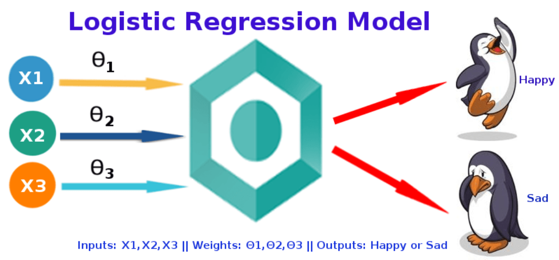
Below is the pictorial representation of a basic logistic regression model to classify set of images into happy or sad.
Both Linear regression and Logistic regression are supervised learning techinques. But for the Regression problem the output is continuous unlike the classification problem where the output is discrete.
- Logistic Regression is used when the dependent variable(target) is categorical.
-
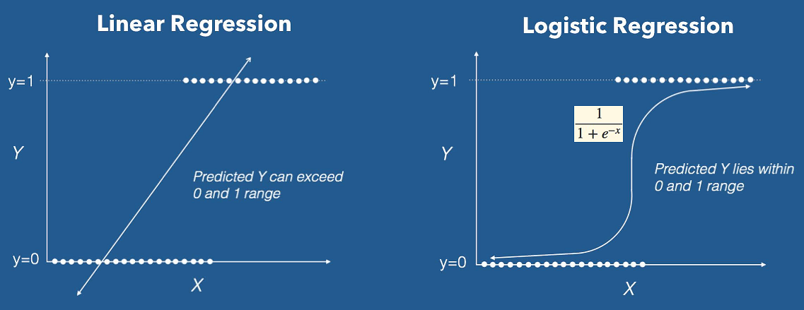
Sigmoid function or logistic function is used as hypothesis function for logistic regression. Below is a figure showing the difference between linear regression and logistic regression, Also notice that logistic regression produces a logistic curve, which is limited to values between 0 and 1.
4.2 Mathematics behind Logistic Regression
The odds for an event is the (probability of an event occuring) / (probability of event not occuring):
 For Linear regression: continuous response is modeled as a linear combination of the features: y = β0 + β1x
For Logistic regression: log-odds of a categorical response being "true" (1) is modeled as a linear combination of the features:
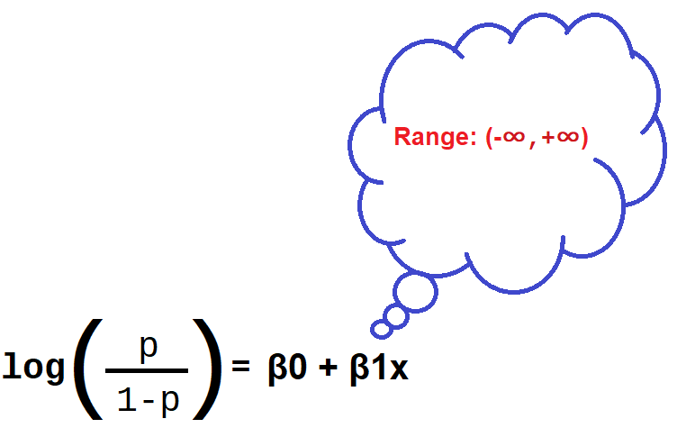 This is called the logit function.
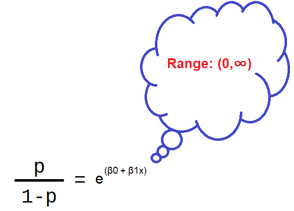
On solving for probability (p) you will get:
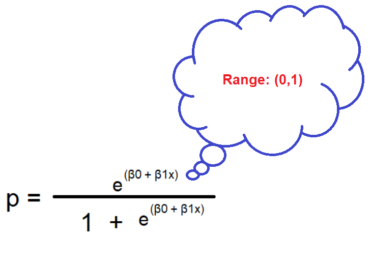
Shown below is the plot showing linear model and logistic model:
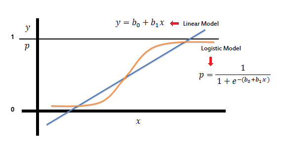
In other words:
- Logistic regression outputs the probabilities of a specific class.
- Those probabilities can be converted into class predictions.
The logistic function has some nice properties:
- Takes on an "s" shape
- Output is bounded by 0 and 1
We have covered how this works for binary classification problems (two response classes). But what about multi-class classification problems (more than two response classes)?
- Most common solution for classification models is "one-vs-all" (also known as "one-vs-rest"): decompose the problem into multiple binary classification problems.
- Multinomial logistic regression can solve this as a single problem.
Logistic Regression was used in biological sciences in early twentieth century. It was then used in many social science applications. For instance,
- The Trauma and Injury Severity Score (TRISS), which is widely used to predict mortality in injured patients, was originally developed by Boyd et al. using logistic regression.
- Many other medical scales used to assess severity of a patient have been developed using logistic regression.
- Logistic regression may be used to predict the risk of developing a given disease (e.g. diabetes; coronary heart disease), based on observed characteristics of the patient (age, sex, body mass index, results of various blood tests, etc.).
Now a days, Logistic Regression have the following applications
- Image segementation and categorization
- Geographic image processing
- Handwriting recognition
- Detection of myocardinal infarction
- Predict whether a person is depressed or not based on a bag of words from corpus.

The reason why logistic regression is widely used despite of the state of the art of deep neural network is that logistic regression is very efficient and does not require too much computational resources, which makes it affordable to run on production.
X = titanic.loc[:,titanic.columns != 'Survived']
X.head()
y = titanic.Survived
from sklearn.model_selection import train_test_split
X_train, X_test, y_train, y_test = train_test_split(X, y, test_size=0.20, random_state=1)
print(X_train.shape)
print(y_train.shape)
To apply any machine learning algorithm on your dataset, basically there are 4 steps:
- Load the algorithm
- Instantiate and Fit the model to the training dataset
- Prediction on the test set
- Calculating the accuracy of the model
The code block given below shows how these steps are carried out:
from sklearn.linear_model import LogisticRegression
    logreg = LogisticRegression()
    logreg.fit(X_train, y_train)
    accuracy_score(y_test,y_pred_test))
from sklearn.linear_model import LogisticRegression
logreg = LogisticRegression()
logreg.fit(X_train,y_train)
y_pred_train = logreg.predict(X_train)
y_pred_test = logreg.predict(X_test) # make predictions on the testing set
- We need an evaluation metric in order to compare our predictions with the actual values.
Error is the deviation of the values predicted by the model with the true values.
We will use accuracy score and confusion matrix for evaluation.
from sklearn.metrics import accuracy_score
print('Accuracy score for test data is:', accuracy_score(y_test,y_pred_test))
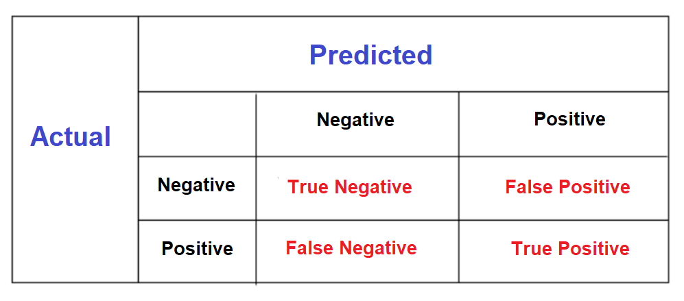
A confusion matrix is a summary of prediction results on a classification problem.
The number of correct and incorrect predictions are summarized with count values and broken down by each class.
Below is a diagram showing a general confusion matrix.
from sklearn.metrics import confusion_matrix

confusion_matrix = pd.DataFrame(confusion_matrix(y_test, y_pred_test))

print(confusion_matrix)
confusion_matrix.index = ['Actual Died','Actual Survived']
confusion_matrix.columns = ['Predicted Died','Predicted Survived']
print(confusion_matrix)
This means 93 + 48 = 141 correct predictions & 25 + 13 = 38 false predictions.
Adjusting Threshold for predicting Died or Survived.
- In the section 4.7 we have used, .predict method for classification. This method takes 0.5 as the default threshhod for prediction.
- Now, we are going to see the impact of changing threshold on the accuracy of our logistic regression model.
- For this we are going to use .predict_proba method instead of using .predict method.
Setting the threshold to 0.75
preds1 = np.where(logreg.predict_proba(X_test)[:,1]> 0.75,1,0)
print('Accuracy score for test data is:', accuracy_score(y_test,preds1))
The accuracy have been reduced significantly changing from 0.79 to 0.73. Hence, 0.75 is not a good threshold for our model.
Setting the threshold to 0.25
preds2 = np.where(logreg.predict_proba(X_test)[:,1]> 0.25,1,0)
print('Accuracy score for test data is:', accuracy_score(y_test,preds2))
The accuracy have been reduced, changing from 0.79 to 0.75. Hence, 0.25 is also not a good threshold for our model.
Later on we will see methods to identify the best threshold.
