LINEAR REGRESSION
A brief introduction to machine learning
- 1. Problem Statement
- 2. Data Loading and Description
- 3. Exploratory Data Analysis
- 4. Introduction to Linear Regression
- 4.1 Linear Regression Equation with Errors in consideration
- 4.2 Preparing X and y using pandas
- 4.3 Splitting X and y into training and test datasets.
- 4.4 Linear regression in scikit-learn
- Linear Regression Model without GridSearcCV
- 4.5 Interpreting Model Coefficients
- 4.6 Using the Model for Prediction
- 5. Model evaluation
- 6. Feature Selection
- 7. Handling Categorical Features
1. Problem Statement
Sales (in thousands of units) for a particular product as a function of advertising budgets (in thousands of dollars) for TV, radio, and newspaper media. Suppose that in our role as Data Scientist we are asked to suggest.
-
We want to find a function that given input budgets for TV, radio and newspaper predicts the output sales.
-
Which media contribute to sales?
-
Visualize the relationship between the features and the response using scatter plots.
2. Data Loading and Description
The adverstising dataset captures sales revenue generated with respect to advertisement spends across multiple channles like radio, tv and newspaper.
- TV - Spend on TV Advertisements
- Radio - Spend on radio Advertisements
- Newspaper - Spend on newspaper Advertisements
- Sales - Sales revenue generated
Importing Packages
import pandas as pd
import seaborn as sns
import matplotlib.pyplot as plt
import warnings
warnings.filterwarnings("ignore")

from sklearn import metrics

import numpy as np

# allow plots to appear directly in the notebook
%matplotlib inline
data = pd.read_csv('Linreg/Advertising.csv', index_col=0)
data.head()
What are the features?
- TV: advertising dollars spent on TV for a single product in a given market (in thousands of dollars)
- Radio: advertising dollars spent on Radio
- Newspaper: advertising dollars spent on Newspaper
What is the response?
- Sales: sales of a single product in a given market (in thousands of widgets)
data.shape
data.info()
data.describe()
There are 200 observations, and thus 200 markets in the dataset.
Distribution of Features
f, axes = plt.subplots(2, 2, figsize=(7, 7), sharex=True)                                      # Set up the matplotlib figure
sns.despine(left=True)

_ = sns.distplot(np.array(data.sales), color="b", ax=axes[0, 0])

_ = sns.distplot(data.TV, color="r", ax=axes[0, 1])

_ = sns.distplot(data.radio, color="g", ax=axes[1, 0])

_ = sns.distplot(data.newspaper, color="m", ax=axes[1, 1])
Observations
Sales seems to be normal distribution. Spending on newspaper advertisement seems to be right skewed. Most of the spends on newspaper is fairly low where are spend on radio and tv seems be uniform distribution. Spends on tv are comparatively higher then spend on radio and newspaper.
JG1 = sns.jointplot("newspaper", "sales", data=data, kind='reg')
JG2 = sns.jointplot("radio", "sales", data=data, kind='reg')
JG3 = sns.jointplot("TV", "sales", data=data, kind='reg')

#subplots migration
f = plt.figure()
for J in [JG1, JG2,JG3]:
    for A in J.fig.axes:
        f._axstack.add(f._make_key(A), A)
Observation
Sales and spend on newpaper is not highly correlaed where are sales and spend on tv is highly correlated.
_=sns.pairplot(data, size = 2, aspect = 1.5)
sns.pairplot(data, x_vars=['TV', 'radio', 'newspaper'], y_vars='sales', size=5, aspect=1, kind='reg')
Observation
- Strong relationship between TV ads and sales
- Weak relationship between Radio ads and sales
- Very weak to no relationship between Newspaper ads and sales
data.corr()
sns.heatmap( data.corr(), annot=True );
Observation
-
The diagonal of the above matirx shows the auto-correlation of the variables. It is always 1. You can observe that the correlation between TV and Sales is highest i.e. 0.78 and then between sales and radio i.e. 0.576.
-
correlations can vary from -1 to +1. Closer to +1 means strong positive correlation and close -1 means strong negative correlation. Closer to 0 means not very strongly correlated. variables with strong correlations are mostly probably candidates for model builing.
4. Introduction to Linear Regression
Linear regression is a basic and commonly used type of predictive analysis. The overall idea of regression is to examine two things:
- Does a set of predictor variables do a good job in predicting an outcome (dependent) variable?
- Which variables in particular are significant predictors of the outcome variable, and in what way they do impact the outcome variable?
These regression estimates are used to explain the relationship between one dependent variable and one or more independent variables. The simplest form of the regression equation with one dependent and one independent variable is defined by the formula :
$y = \beta_0 + \beta_1x$

What does each term represent?
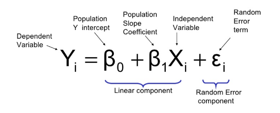
- $y$ is the response
- $x$ is the feature
- $\beta_0$ is the intercept
- $\beta_1$ is the coefficient for x
Three major uses for regression analysis are:
- determining the strength of predictors,
- Typical questions are what is the strength of relationship between dose and effect, sales and marketing spending, or age and income.
-
forecasting an effect, and
- how much additional sales income do I get for each additional $1000 spent on marketing?
-
trend forecasting.
- what will the price of house be in 6 months?
4.1 Linear Regression Equation with Errors in consideration
While taking errors into consideration the equation of linear regression is:
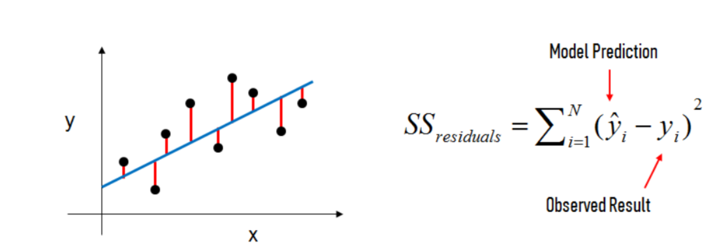
 Generally speaking, coefficients are estimated using the least squares criterion, which means we are find the line (mathematically) which minimizes the sum of squared residuals (or "sum of squared errors"):
What elements are present in the diagram?
- The black dots are the observed values of x and y.
- The blue line is our least squares line.
- The red lines are the residuals, which are the distances between the observed values and the least squares line.

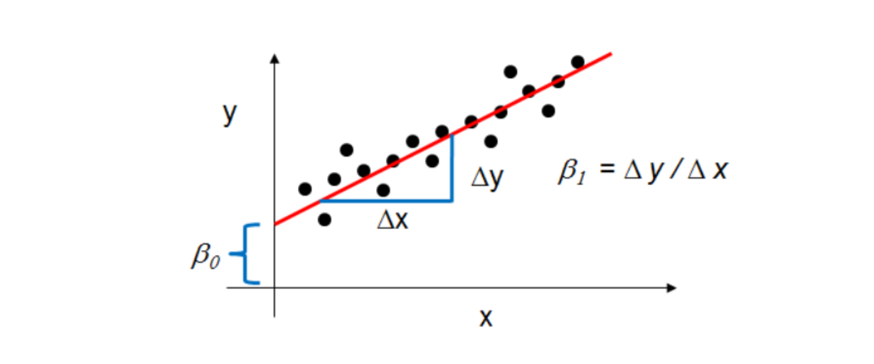
How do the model coefficients relate to the least squares line?
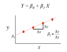
- $\beta_0$ is the intercept (the value of $y$ when $x$ = 0)
- $\beta_1$ is the slope (the change in $y$ divided by change in $x$)
Here is a graphical depiction of those calculations:

- There should be a linear and additive relationship between dependent (response) variable and independent (predictor) variable(s). A linear relationship suggests that a change in response Y due to one unit change in X¹ is constant, regardless of the value of X¹. An additive relationship suggests that the effect of X¹ on Y is independent of other variables.
- There should be no correlation between the residual (error) terms. Absence of this phenomenon is known as Autocorrelation.
- The independent variables should not be correlated. Absence of this phenomenon is known as multicollinearity.
- The error terms must have constant variance. This phenomenon is known as homoskedasticity. The presence of non-constant variance is referred to heteroskedasticity.
- The error terms must be normally distributed.
-
Standardization.
Standardize features by removing the mean and scaling to unit standard deviation.
from sklearn.preprocessing import StandardScaler
scaler = StandardScaler().fit(data)
data1 = scaler.transform(data)
data = pd.DataFrame(data1)
data.head()
data.columns = ['TV','radio','newspaper','sales']
data.head()
feature_cols = ['TV', 'radio', 'newspaper']                # create a Python list of feature names
X = data[feature_cols]                                     # use the list to select a subset of the original DataFrame-+
- Checking the type and shape of X.
print(type(X))
print(X.shape)
y = data.sales
y.head()
- Check the type and shape of y
print(type(y))
print(y.shape)
from sklearn.model_selection import train_test_split

def split(X,y):
    return train_test_split(X, y, test_size=0.20, random_state=1)
X_train, X_test, y_train, y_test=split(X,y)
print('Train cases as below')
print('X_train shape: ',X_train.shape)
print('y_train shape: ',y_train.shape)
print('\nTest cases as below')
print('X_test shape: ',X_test.shape)
print('y_test shape: ',y_test.shape)
To apply any machine learning algorithm on your dataset, basically there are 4 steps:
- Load the algorithm
- Instantiate and Fit the model to the training dataset
- Prediction on the test set
- Calculating Root mean square error
The code block given below shows how these steps are carried out:
from sklearn.linear_model import LinearRegression
    linreg = LinearRegression()
    linreg.fit(X_train, y_train)
    RMSE_test = np.sqrt(metrics.mean_squared_error(y_test, y_pred_test))
def linear_reg( X, y, gridsearch = False):

    X_train, X_test, y_train, y_test = split(X,y)

    from sklearn.linear_model import LinearRegression
    linreg = LinearRegression()

    if not(gridsearch):
        linreg.fit(X_train, y_train)

    else:
        from sklearn.model_selection import GridSearchCV
        parameters = {'normalize':[True,False], 'copy_X':[True, False]}
        linreg = GridSearchCV(linreg,parameters, cv = 10,refit = True)
        linreg.fit(X_train, y_train)                                                           # fit the model to the training data (learn the coefficients)
        print("Mean cross-validated score of the best_estimator : ", linreg.best_score_)

        y_pred_test = linreg.predict(X_test)                                                   # make predictions on the testing set

        RMSE_test = np.sqrt(metrics.mean_squared_error(y_test, y_pred_test))                          # compute the RMSE of our predictions
        print('RMSE for the test set is {}'.format(RMSE_test))

    return linreg
X = data[feature_cols]
y = data.sales
linreg = linear_reg(X,y)
print('Intercept:',linreg.intercept_)          # print the intercept
print('Coefficients:',linreg.coef_)
Its hard to remember the order of the feature names, we so we are zipping the features to pair the feature names with the coefficients
feature_cols.insert(0,'Intercept')
coef = linreg.coef_.tolist()
coef.insert(0, linreg.intercept_)
eq1 = zip(feature_cols, coef)

for c1,c2 in eq1:
    print(c1,c2)
y = 0.00116 + 0.7708 * TV + 0.508 * radio + 0.010 * newspaper
How do we interpret the TV coefficient (0.77081)
- A "unit" increase in TV ad spending is associated with a "0.7708 unit" increase in Sales.
- Or more clearly: An additional $1,000 spent on TV ads is associated with an increase in sales of 770.8 widgets.
Important Notes:
- This is a statement of association, not causation.
- If an increase in TV ad spending was associated with a decrease in sales, β1 would be negative.
y_pred_train = linreg.predict(X_train)
y_pred_test = linreg.predict(X_test) # make predictions on the testing set
- We need an evaluation metric in order to compare our predictions with the actual values.
Error is the deviation of the values predicted by the model with the true values.
For example, if a model predicts that the price of apple is Rs75/kg, but the actual price of apple is Rs100/kg, then the error in prediction will be Rs25/kg.
Below are the types of error we will be calculating for our linear regression model:
- Mean Absolute Error
- Mean Squared Error
- Root Mean Squared Error
Mean Absolute Error (MAE) is the mean of the absolute value of the errors: $$\frac 1n\sum_{i=1}^n|y_i-\hat{y}_i|$$ Computing the MAE for our Sales predictions
MAE_train = metrics.mean_absolute_error(y_train, y_pred_train)
MAE_test = metrics.mean_absolute_error(y_test, y_pred_test)
print('MAE for training set is {}'.format(MAE_train))
print('MAE for test set is {}'.format(MAE_test))
Mean Squared Error (MSE) is the mean of the squared errors: $$\frac 1n\sum_{i=1}^n(y_i-\hat{y}_i)^2$$
Computing the MSE for our Sales predictions
MSE_train = metrics.mean_squared_error(y_train, y_pred_train)
MSE_test = metrics.mean_squared_error(y_test, y_pred_test)
print('MSE for training set is {}'.format(MSE_train))
print('MSE for test set is {}'.format(MSE_test))
Root Mean Squared Error (RMSE) is the square root of the mean of the squared errors:
$$\sqrt{\frac 1n\sum_{i=1}^n(y_i-\hat{y}_i)^2}$$
Computing the RMSE for our Sales predictions
RMSE_train = np.sqrt( metrics.mean_squared_error(y_train, y_pred_train))
RMSE_test = np.sqrt(metrics.mean_squared_error(y_test, y_pred_test))
print('RMSE for training set is {}'.format(RMSE_train))
print('RMSE for test set is {}'.format(RMSE_test))
Comparing these metrics:
- MAE is the easiest to understand, because it's the average error.
- MSE is more popular than MAE, because MSE "punishes" larger errors.
-
RMSE is even more popular than MSE, because RMSE is interpretable in the "y" units.
- Easier to put in context as it's the same units as our response variable.
- There is one more method to evaluate linear regression model and that is by using the Rsquared value.
-
R-squared is the proportion of variance explained, meaning the proportion of variance in the observed data that is explained by the model, or the reduction in error over the null model. (The null model just predicts the mean of the observed response, and thus it has an intercept and no slope.)
-
R-squared is between 0 and 1, and higher is better because it means that more variance is explained by the model. But there is one shortcoming of Rsquare method and that is R-squared will always increase as you add more features to the model, even if they are unrelated to the response. Thus, selecting the model with the highest R-squared is not a reliable approach for choosing the best linear model.
There is alternative to R-squared called adjusted R-squared that penalizes model complexity (to control for overfitting).
yhat = linreg.predict(X_train)
SS_Residual = sum((y_train-yhat)**2)
SS_Total = sum((y_train-np.mean(y_train))**2)
r_squared = 1 - (float(SS_Residual))/SS_Total
adjusted_r_squared = 1 - (1-r_squared)*(len(y_train)-1)/(len(y_train)-X_train.shape[1]-1)
print(r_squared, adjusted_r_squared)
yhat = linreg.predict(X_test)
SS_Residual = sum((y_test-yhat)**2)
SS_Total = sum((y_test-np.mean(y_test))**2)
r_squared = 1 - (float(SS_Residual))/SS_Total
adjusted_r_squared = 1 - (1-r_squared)*(len(y_test)-1)/(len(y_test)-X_test.shape[1]-1)
print(r_squared, adjusted_r_squared)
6. Feature Selection
At times some features do not contribute much to the accuracy of the model, in that case its better to discard those features.
- Let's check whether "newspaper" improve the quality of our predictions or not.
To check this we are going to take all the features other than "newspaper" and see if the error (RMSE) is reducing or not. - Also Applying gridsearch method for exhaustive search over specified parameter values of estimator.
feature_cols = ['TV','radio']                                                          # create a Python list of feature names
X = data[feature_cols]
y = data.sales
linreg=linear_reg(X,y,gridsearch=True)
-
Before doing feature selection RMSE for the test dataset was 0.271182.
-
After discarding 'newspaper' column, RMSE comes to be 0.268675.
- As you can see there is no significant improvement in the quality, therefore, the 'newspaper' column shouldn't be discarded. But if in some other case if there is significant decrease in the RMSE, then you must discard that feature.
- Give a try to other features and check the RMSE score for each one.
np.random.seed(123456)                                                # set a seed for reproducibility
nums = np.random.rand(len(data))
mask_suburban = (nums > 0.33) & (nums < 0.66)                         # assign roughly one third of observations to each group
mask_urban = nums > 0.66
data['Area'] = 'rural'
data.loc[mask_suburban, 'Area'] = 'suburban'
data.loc[mask_urban, 'Area'] = 'urban'
data.head()
We want to represent Area numerically, but we can't simply code it as:
- 0 = rural,
- 1 = suburban,
- 2 = urban
Because that would imply an ordered relationship between suburban and urban, and thus urban is somehow "twice" the suburban category.
Note that if you do have ordered categories (i.e., strongly disagree, disagree, neutral, agree, strongly agree), you can use a single dummy variable to represent the categories numerically (such as 1, 2, 3, 4, 5).
Anyway, our Area feature is unordered, so we have to create additional dummy variables. Let's explore how to do this using pandas:
area_dummies = pd.get_dummies(data.Area, prefix='Area')                           # create three dummy variables using get_dummies
area_dummies.head()
However, we actually only need two dummy variables, not three. Why??? Because two dummies captures all the "information" about the Area feature, and implicitly defines rural as the "baseline level".
Let's see what that looks like:
area_dummies = pd.get_dummies(data.Area, prefix='Area').iloc[:, 1:]
area_dummies.head()
Here is how we interpret the coding:
- rural is coded as Area_suburban = 0 and Area_urban = 0
- suburban is coded as Area_suburban = 1 and Area_urban = 0
- urban is coded as Area_suburban = 0 and Area_urban = 1
If this sounds confusing, think in general terms that why we need only k-1 dummy variables if we have a categorical feature with k "levels".
Anyway, let's add these two new dummy variables onto the original DataFrame, and then include them in the linear regression model.
data = pd.concat([data, area_dummies], axis=1)
data.head()
feature_cols = ['TV', 'radio', 'newspaper', 'Area_suburban', 'Area_urban']             # create a Python list of feature names
X = data[feature_cols]
y = data.sales
linreg = linear_reg(X,y)
feature_cols.insert(0,'Intercept')
coef = linreg.coef_.tolist()
coef.insert(0, linreg.intercept_)

eq1 = zip(feature_cols, coef)

for c1,c2 in eq1:
    print("{} : {}".format(c1.rjust(15," "),c2))
y = - 0.00218 + 0.7691 * TV + 0.505 * radio + 0.011 * newspaper - 0.0311 * Area_suburban + 0.0418 * Area_urban
How do we interpret the coefficients?
- Holding all other variables fixed, being a suburban area is associated with an average decrease in Sales of 0.0311 widgets (as compared to the baseline level, which is rural).
- Being an urban area is associated with an average increase in Sales of 0.0418 widgets (as compared to rural).